Measuring and Improving Cooling System Performance – Part 4: Heat Exchanger
A "heat exchanger" is, as the name suggests, a device for transferring energy
from one working fluid to another. Here, we want to transfer internal energy
from the liquid coolant to air; this transfer process is called "heat." If we
input enough heat, we can use the increased energy of the air to generate
thrust; this is basically what jet engines do. However, we're constrained in
designing or modifying a road car by low mass flow. While a car cooling system
can ingest a few pounds of air each second, a GEnx-2B67 engine on the 747-8,
for example, swallows more than one ton per second at takeoff (that's per
engine—747s have to move a lot of air to get off the ground!).
Additionally, small temperature differences and tight engine packaging will
make it difficult to get thrust/negative drag overall—even in the best case,
the theoretical maximum thrust is very, very small. A better goal is simply to
minimize drag from the cooling system, which we'll look at more in later posts.
 |
| Due to packaging constraints, there often isn't a lot of room to work with behind or around the heat exchanger. Sometimes, clever packaging is used to increase core area, as on this BMW M5 with an exchanger placed horizontally just behind the inlet. |
Heat
Exchanger: State 2 to State 3
To
build a mathematical model of heat exchanger flow we'll add two more
conservation equations. As before, conservation of mass applies—so, assuming
steady state, we'll have a constant mass flow through the exchanger and, approximating
its inlet and exit streamtube areas as the same (we'll investigate the veracity
of this later),

Note
that the mass flow per area here is different than what I plotted in the first
post in this series; that was mass flow per unit inlet area. To find
that for a core of a given size, simply multiply your inlet mass flow by the velocity
ratio you measured in Part 3:

Conservation
of Momentum
Next,
let's apply conservation of momentum (Navier-Stokes equations) to determine the
force acting on the heat exchanger. Just like mass, momentum must be conserved
and cannot spontaneously be created or destroyed within a control volume:

As
before, we'll assume steady state operation; we'll also assume body forces
(e.g. gravity, the last term above) acting on the air are negligible,
one-dimensional flow, and a control volume that follows the external outline of
the exchanger. Solving the remaining integrals gives us the drag force on the
exchanger (which arises from all internal forces the fluid exerts; here, that
consists solely of the friction over its wetted surfaces if we approximate the
fin area normal to the flow direction as negligible),

with
positive axial direction defined in the direction of the drag force. (If you're
familiar with the thrust equation, that’s basically what this is, turned around
so it gives drag as a positive value—it derives directly from conservation of
momentum).
In
cooling system design, it is common to approximate flow velocity through the
core as a constant. This is not really correct; applying conservation of mass,
along with the fact that the density of the hotter airflow out of the heat
exchanger will be less than the density of the cooler airflow in, shows that either u3
> u2 or streamtube area A3 > A2,
or some combination of both. We’ll revisit this idea in just a minute, when we
measure dynamic pressure at the heat exchanger outlet and later on when we test
a physical model of a ducted heat exchanger that visibly illustrates this
phenomenon, and see what the implications are. For now, we can assume that u2
≈ u3 ≈ ucore for simplicity's sake. If we apply this
approximation, then the equation above becomes:

…and
total pressure loss across the core is equal to static pressure loss. A common
point of confusion (that I wasn't even clear on until I
worked through all this): although they are related and vary together, it is total pressure loss, not static
pressure loss, across the core that increases or decreases cooling
capacity—we’ll see why in just a minute.
Conservation
of Energy
Finally,
we reach the crux of the heat exchanger model: the energy balance. Like mass
and momentum, energy cannot be created or destroyed—so all the energy that
comes into our system must be accounted for on its way out. Assuming again that
our car is operating at steady state so the time derivative terms drop out, and
neglecting body forces,

The
first term here tells us the convection of energy (energy carried along by the
flow in the form of total enthalpy h0, which includes the
ability to do pressure work and the kinetic energy of the flow); the second
term is energy in the friction/shear stresses along the wetted surface
area/walls; and the third term is the heat added from the coolant. At low
temperature and pressure we can approximate enthalpy using a calorically
perfect model,

where
cp is the constant pressure specific heat, about 1.004
kJ/kg-K for standard air (don't confuse this with the other CP,
static pressure coefficient!). This gives us the solution for cooling capacity,

Let's
rearrange this equation to show more clearly what's going on:

On
the left-hand side we have energy coming into the heat exchanger, and on the
right-hand side, energy going out. At steady state (e.g. your car driving at
constant speed after it has warmed up) these should be equal; if the energy
going out is less than coming in, your car will overheat. We need these to be
matched, ideally in all environments and driving conditions but realistically
in the worst-case scenario of hot weather (small ΔT), high engine load
(large Q), and low speed (small ṁ).
On
the left we have the static enthalpy of the air going in, its kinetic energy,
and the energy added from the coolant as heat, by conduction through the
exchanger walls and convection in the boundary layer (a small amount by
radiation, but conduction and convection dominate). On the right are the static
enthalpy of the air coming out, its kinetic energy, and the energy lost to
dissipation in the heat exchanger flow i.e. friction effects in the boundary
layer (plus some small amount radiated away).
Let's
go through this one side at a time. We can't really do anything about the heat
coming in, since that's a function of the powertrain and is what it is for any
given engine operating condition and load. Similarly, we're at the mercy of
environmental conditions to determine the mass-specific enthalpy cpT
of the air coming in since this is related to its temperature. But we can
do something about the mass flow rate ṁ: reducing this will reduce both
the enthalpy and kinetic energy of the airflow in. Further, we can reduce the
kinetic energy coming in by reducing u2, the speed of airflow
into the heat exchanger.
Ideally,
we'll turn all that energy into enthalpy in the airflow out but realistically
this can’t happen (if it could, we would have a zero-drag exchanger—an obvious
impossibility). The airflow out will also have some kinetic energy, and energy
will be lost to dissipation inside the heat exchanger. You should see a problem
now with decreasing ṁ: our main sources of energy removal are also
proportional to mass flow, so reducing it will reduce your car’s cooling
capacity.
Again
applying an assumption that u2 ≈ u3 ≈ ucore,
the kinetic energy terms drop out (i.e. all the kinetic energy coming in also
leaves as kinetic energy) and we are left with,

…or,
rearranged to solve for heat dissipation:

So
we see that heat dissipation, or cooling capacity, is proportional to the mass
flow through the cooling system, the temperature difference between the air in
and air out, and power losses in boundary layer friction within the heat
exchanger. These losses are proportional to the total pressure loss (energy
dissipation) across the core; increasing total pressure loss in the heat
exchanger takes more energy out of the flow and thus increases cooling
capacity. These losses are due to friction in the flow over the heat exchanger
walls, which is inversely proportional to the flow velocity into the exchanger
(since friction coefficient is inversely proportional to Reynolds number). For
a heat exchanger with a fixed wetted internal area and assuming turbulent flow
throughout, this means that total pressure loss is proportional to ucore1.8
because,

So,
total pressure loss through the heat exchanger is reduced if we reduce the
velocity of the flow going into it. For any heat exchanger, there will be a ucore—and,
by extension, Ain and Aout streamtube areas—to
which the flow will naturally conform in the absence of ducting. Can we predict
those areas?
Loss
Coefficient ξcore
The
answer to that is "yes," since it is related to the loss coefficient
across the core, where

(That's
the Greek letter "xi." We’ve seen this before, implicitly, in the equation for diffuser
efficiency in Part 3). This loss coefficient is the heat exchanger drag
coefficient, referenced to core area (you can prove this yourself using the approximated
result of the momentum balance above). According to the literature, most
passenger cars have heat exchangers with loss coefficients between 4-10. The
higher the loss coefficient, the less mass flow is needed to achieve the same
cooling capacity since a higher loss coefficient means more energy is removed
from the coolant and dissipated in boundary layer friction within the heat
exchanger. This tells us how large the inlet and outlet streamtubes should be,
referenced to exchanger core area, for a "free" (unducted) heat exchanger with
given loss coefficient (and, thus, the required inlet and outlet sizes of a fully ducted
system for maximum cooling capacity):

Free
heat exchangers should have a core velocity that is a function of loss coefficient:

Notice
that loss coefficient goes down with increases in ucore.
Don’t be confused by this! While the drag coefficient of the exchanger
core goes down with increasing ucore, the drag force
on the exchanger goes up (since it is proportional to ucore1.8,
as derived above).
Ducted
systems with an outlet smaller than shown above will have restricted mass flow and a smaller inlet capture area. These ducted exchangers should have a core velocity
that varies with loss coefficient and outlet area:

Loss
coefficient is a function of the physical design of the heat exchanger,
especially its internal surface area (Swet in the equation
above) which can be on the order of 100 times larger than core area, and the
velocity of the flow into it. As such, it varies inversely with ucore/u∞
and you can also change it by swapping in a heat exchanger of a different size
or design (especially number of fins per inch; as fins per inch goes down, so does Swet).
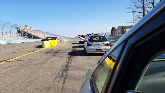
Testing
Now,
let's see if we can actually calculate ξcore on our own cars. We
can do that by finding the total pressure loss across the heat exchanger
package and the dynamic pressure of the flow through the heat exchanger.
First,
let's find dynamic pressure q2 the same way as last time.
Tape a pressure disk and a tube end to the heat exchanger face. Then measure
the gauge pressure between them; this is the direct value of q2.
 |
| When you're taking measurements at multiple locations, be careful with your tubing management. Route them with minimal distortion to the car body shape, and label each tube end inside the car for easy and efficient connection to your manometer during testing. |
Next,
measure the total pressure loss across the exchanger package. Use the same
pressure disk taped to the front of it but now record gauge pressure relative
to a total probe (tube facing forward) behind the heat exchanger. Place the
tube opening as close to the back of the heat exchanger as possible; if your
car has electric cooling fans and you know at what coolant temperature they
activate (on my car, that's 202°F), you may be able to stick the tube between
the blades so long as you know the fans will stay off. However, it's a close
enough approximation to take a reading just behind the fans, which tend to be
placed right up against the exchanger outlet anyway. Alternatively, you can
drill a small hole in the fan shroud (which you can plug later).

Then,
using a static probe/tube end taped in place onto or behind the fan shroud (or
inserted through a hole drilled into the top or side of the shroud), record the
difference between total pressure and static pressure behind the heat exchanger
to get q3.
Let's
compare q2 and q3. We know from our
analysis above that even if u2 ≈ u3, ρ2
≠ ρ3 due to the change in enthalpy as airflow passes through
the core and the dynamic pressures cannot be equal. How close are they?

Not
even close. In fact, at 45 mph vehicle speed, q3 was so small
it wasn’t measurable, and at all speeds the dynamic pressure at the heat
exchanger outlet is a small fraction of the inlet value. We'll revisit this and
determine its implications in a later post.
Calculate
ξcore by dividing the total
pressure loss by dynamic pressure qcore. We'll approximate qcore
as the average of q2 and q3 (in the
literature, core flow speed is considered constant but it clearly is not in
real life! So we'll take qcore as the average of inlet and
outlet dynamic pressure) giving loss coefficient:

If
you test at lower speeds than I did, you may find more variation in loss
coefficient. As heat exchanger inlet flow speed increases, you should find that
ξcore converges to approximately
constant (this happens as the internal flow becomes fully turbulent). Here, it
looks like loss
coefficient ξcore ≈ 4 on my car—on the low end of expected values. Similar to the
high ucore/u∞ I found in previous testing, this
indicates high internal drag from the cooling system (recall from our analysis
above that loss coefficient goes up with decreasing velocity ratio but drag
goes down. The relationship between ξcore and drag force
is an inverse one). Also, if you look at the velocity plot for an unducted
radiator above, you will see that the loss coefficient I found here corresponds
almost exactly to the velocity ratio I measured in Part 3. Everything I've
measured so far seems to indicate that there is room for significant
improvement of my car's cooling system.
Finally,
you can use your measurement data to calculate static pressure loss across the
core and compare to total pressure loss by,

…with
the deltas here defined as upstream minus downstream to give the correct sign. Heat
exchanger analyses in sources like Barnard and Hoerner assume static pressure
loss equal to total pressure loss, but reality shows:

On my car, static pressure loss is about half of total
pressure loss. Since
cooling capacity is dependent on total pressure loss, be careful about
what you’re actually measuring; in the past, I wrote that the "amount" of flow (a term that isn’t really meaningful since it is too imprecise) is dependent on static pressure loss but that doesn't give us the
whole picture. If you want to characterize the performance of the heat
exchanger(s) on your car, you should measure total pressure loss and dynamic
pressure in and out of the exchanger; those parameters will tell you far more
about the flow velocity through the heat exchanger package and cooling capacity
than static pressure loss alone. We'll revisit this later on, when we test a
physical heat exchanger model and compare it to the real one under the hood.
Heat
Exchanger Area and Drag
Before
we go on to the fans and outlet in the next post, just a quick comment on
internal drag. A lot of people wonder why EVs use such large heat exchangers,
and a few even think they don't need cooling at all. This is not even close to
true; batteries and electric motors generate waste heat because no process is
ideal, and this energy has to go somewhere if you don't want the powertrain to
degrade over time (something early Nissan Leaf owners know all too well). Batteries and electric motors also tend to have narrower
temperature range tolerances than combustion engines, so adequate cooling capacity and system performance are as critical as on combustion engine cars.
We
can assume, however, that the necessary cooling capacity of an electric
powertrain is less than that of a combustion engine because of its higher
thermal efficiency. Why, then, use a large heat exchanger? It's because, for
the same mass flow rate and cooling requirement, a large exchanger will have less
internal drag than a smaller one.
There
are a variety of ways to prove this mathematically; perhaps the most intuitive
is Hoerner's explanation (part of which I've derived for you above: the
relationship between total pressure loss and ucore). Since
drag on the heat exchanger is proportional to the flow velocity into it, reduce
ucore and drag goes down. For some required ṁ, the
only way to reduce ucore is by increasing Acore
(recall the "area rule" we derived from the continuity equation in the last
post). Further, because Acore and ucore are
directly proportional but total pressure loss is proportional to ucore1.8,
the benefit of lower core velocity outweighs the drag increase from a larger core
area. Hence, the larger heat exchanger has less drag than the smaller one. Look
at the cooling system of any EV to see this phenomenon in action.
 |
| Take this 2026 Jeep Recon, for example. It has a cooling package similar in size and design to a combustion-powered car despite having a lower cooling requirement (which we can tell from the relatively small inlet area). Why? Because this results in lower drag than a smaller heat exchanger. |
You
can see this on combustion-powered cars as well. As engines have become more
efficient (I'll write more on efficiency and how to measure it in a future
post), heat exchangers have not shrunk—they're bigger, in fact. My old truck,
for instance, has a 22R-E engine that has lower thermal efficiency than the
2ZR-FXE in my Prius and much higher vehicle road load, so it produces more
waste heat. But the truck has a heat exchanger that is slightly smaller than
the engine heat exchanger in the Prius: 2.15 ft2 on the former
compared to 2.41 ft2 on the latter,
making the diffuser outlet area larger for lower ucore
and less drag. Further, looking up the part dimensions online shows that the engine heat exchanger has continued to grow on succeeding generations of Prius: from 2.41 ft2 on the third generation (2010) to 2.68 ft2 on the fourth (2016), and 3.01 ft2 on the fifth (2023).
Next time: outlets.


Comments
Post a Comment