How to Estimate Your Car's Coefficient of Rolling Resistance

When two objects in contact with each other slide, a friction force develops resisting the motion. In classical physics, we distinguish between static friction (which resists the onset of motion as some force is applied) and kinetic friction (which resists movement after it has begun). You’ve noticed this before: the last time you tried to push a heavy box across the floor, say, you had to give it a push to get started and overcome the static friction (and if the static friction was great enough, it perhaps tipped over instead of sliding). When you stopped pushing, it didn’t continue sliding indefinitely; it gradually slowed and required some force to keep moving (although not as much as it took to get started). In both scenarios, your pushing on the box was required to overcome its static or kinetic friction.

Upright, the fluid-filled can slides when pushed but as energy is dissipated due to friction with the table surface, it quickly comes to a stop.

Cars are a bit more complicated because most of the time the tires don’t just slide relative to the ground, they roll as well. So, to model the resistance force that opposes a car’s motion due to its contact with the road we don’t use simple friction but rolling resistance. This approximates not just the tires’ friction with the road but also the tendency of all the spinning things on the car—tires, wheels, brake rotors, wheel bearings, axles, transmission components—to not want to rotate due to their angular inertia and internal friction.

On its side, the same can rolls easily with far less force applied despite having the same mass as before. You should deduce from this experiment that rolling resistance coefficients are much smaller than friction coefficients for most objects (including cars).

Similar to the historical derivation of the model equation for aerodynamic drag (over time, scientists deduced from measurement that drag was proportional to the square of velocity, fluid density, etc.), we know from centuries of empirical data that the rolling resistance of wheeled objects such as cars is proportional to their weight. Mathematically,

…where C_RR is a proportionality constant called the “coefficient of rolling resistance.” C_RR of a typical car on smooth pavement is generally in the range 0.010-0.020 and for most purposes can be estimated based on what type of tire is on the car: LRR tires on the low end, non-LRR highway all-seasons in the middle, softer summer tires and all-terrains at the high end.

 
What if you want to get a more realistic estimate of C_RR for your specific car, or see how it changes with differences in, say, tire pressure? This was on my mind a few weeks ago so I thought I would devise a test to measure it.
 
Initial Idea
 
My first thought was to try and calculate rolling resistance from a coast down test.
 
Where a coast down test to measure changes in aerodynamic drag relies on an assumption of high speed (so that aero drag is much larger than rolling drag), if we want to measure rolling resistance and minimize the effect of aero drag we should do the opposite: coast down at very low speed.
 
How low? Low enough that the magnitude of aerodynamic drag is very small in comparison to rolling drag yet high enough that the test still gives us easily measurable acceleration without taking forever (and potentially introducing more error over a longer test).
 
To determine what might be a good speed range for this test, do some quick calculations. First, rolling drag is easy enough to figure out since it is not dependent on speed (in this simplified concept; in reality, there will be some dependency since it is influenced by the friction in spinning bearings, deformation and hysteresis in the tires, angular momentum of rotating components etc.).

(You might notice I’ve changed weight here to “effective weight,” as some SAE textbooks suggest. This is an estimated weight based on addition of some penalty, usually 2-3%, to account for the angular inertial moments I mentioned above. We’ll see below that this does not matter for purposes of the testing I’ve developed here).

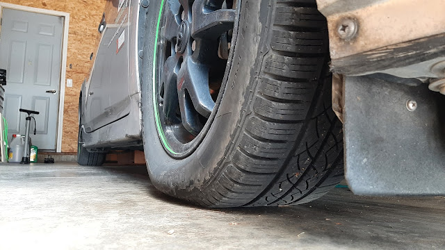Sidewall bulge becomes more pronounced as tire pressure is reduced, increasing rolling resistance as the tire deforms more through each rotation. This can be hard to spot visually (for example, this tire has been aired down to just 20 psi), so be sure to check your tire pressures regularly.

Second, aerodynamic drag is proportional to the square of velocity.

Plot both as a function of velocity and you can see where a good speed range might be if you want to minimize or maximize the effect of one or the other on measurements:

The sum of these, marked in green, is the “road load” plot for my car, or the resistance force it must counter to drive at any speed.

You can also plot road load horsepower rather than force:

Look at old SAE papers and you can find lots of these graphs, many evaluated and drawn by hand. Here’s the road load power graph of the original Ford GT, with its engine output and predicted top speed (actual top speed was significantly lower, 197 mph, due to the drag from internal ducting in the real car):

From SAE 670065, “Development of Ford GT Sports-Racing Car.” Read this paper if you want to get an idea of how much of the engineering process depicted in Ford v. Ferrari was left out or blatantly misrepresented, especially its aerodynamics engineering (spoiler: it was a lot). You get a prize if you can spot the anomaly in this graph (see the end of this post for the answer).

We see on the first graph that rolling drag equals aero drag at around 51 mph on my car (using an assumed rolling resistance coefficient for now). At 16 mph, aero drag is about 10% as much as rolling drag. At 10 mph aero drag is less than 4% of rolling drag and at 5 mph it’s less than 1% of rolling drag. Less than 5% seems small enough to consider negligible for this experiment (this is the sort of “engineering judgment” we have to make in practice all the time) while allowing sufficient speed range to measure velocity over time and calculate acceleration. This modifies our model equation for the force acting on the car to

Rearranging and substituting, we solve for C_RR:

Et voilá: a formula for calculation of C_RR from experimental data.
 
Reality Bites
 
I searched in vain for a stretch of road long enough (~300 ft or longer for my Prius), flat enough, and level enough to do this test. You can check for these by coasting your car at low speed in both directions on a candidate road. If it holds speed or speeds up in one direction and slows in the other, the road is not level. If it speeds up and slows down in the same direction, the road is not flat. To use this test, you will need a perfectly flat, perfectly level road; any slope or undulation at all will induce a drag or thrust force on the car larger than the rolling resistance we’re trying to measure.
 
No matter where I tried, no road around here proved to be suitable. Even smooth parking lots I thought might work turned out to have measurable slope or undulations. In the end, I gave up. Oh well, it was a nice idea in theory. You might have better luck, especially if you have access to something like an airport runway or automotive test track.
 
A Simpler Method
 
The failure of my initial method to pan out prompted me to consider other ways in which a person might measure the rolling resistance of their car at home. Finally, it dawned on me and, after several rounds of testing and fiddling with the procedure, I came up with the following.
 
To do this, you simply need a small space—like a parking spot or a garage—that has a slight slope to it, with enough room to let your car roll a few feet. After warming up your car by driving it for a while, stop in the parking spot with the nose toward the downhill direction. Then shift to neutral, lift your foot off the brake pedal, and observe whether the car begins rolling forward or not. Before or after doing the roll test, measure the slope of the pavement. Take the sine of that angle: if your car rolled, this value is greater than C_RR, and if it didn’t roll, it is less than or equal to C_RR.
 
The warmup is important because C_RR is not constant, even if approximating it as such is usually good enough for predicting performance (as in the plots above). For example, I tried this with my truck in the garage first thing the other morning. Cold, it did not roll, which means it had C_RR > 0.019, based on the slope of the floor on that side of the garage. After running some errands around town, I tried it again with the truck warm. This time, it rolled—so, C_RR < 0.019. I’ll have to wait until winter to try this in different ambient temperatures, but I expect to find seasonal variation based on outside air temperature as well.
 
How does this work, physically? Since weight always acts vertically, on an incline there will be a weight component along the car’s horizontal body axis trying to move it. If this weight component is smaller than the rolling resistance, the car won’t move; if it is larger, the car will roll. The body-frame horizontal weight component, W_x, is given by

…and F_RR as above by

So, for the car to move:

But we can do better. If the car moves, it will accelerate from its resting state. We can model this acceleration mathematically by relating it to the two opposing forces:

Giving:

(Note the similarity between this and the equation we derived in the first part for C_RR: they are identical apart from the sine term, which is simply an artifact of the slope).
 
Thus, if we can measure the acceleration of the car then it should be possible to calculate C_RR. You can do this using an app on your smartphone like Physics Toolbox or another that can read the phone’s accelerometer. Open the app and slide the phone in various directions to determine which is the x-axis, which the y-axis, and which the z-axis. Looking at the screen on my phone, +x is to the left side, +y to the top, and +z out the back. The relationship between these axes follows the right-hand rule and should be the same on any phone (because any one axis is the cross product of the other two, or the vector orthogonal to both), so once you determine the positive direction of two axes you can find the last pretty easily.
 
In the car, align one of the phone’s axes with the car’s longitudinal body axis. I chose to use x, following aerospace convention (+x out the front of the car, +y to the right, and +z down) by taping the phone to the dash sideways after checking that it showed the same angle as the floor. It's important that the phone be fixed to the car as securely as possible. Any relative movement between the phone and car will show up in the measured acceleration, as I found in initial testing (you can still see it in the plots below as a negative spike when the car begins rolling and a corresponding positive spike when the brake is applied). It's impossible to eliminate this, but try and minimize it as much as possible by taping the phone down or otherwise fixing it to the car. We're trying to measure the car's acceleration here, not the phone's.

Set the app to show linear acceleration and record the axis that aligns with the car’s motion. If the app allows calibration, do that now to zero out the accelerometer while the car is at rest. Then, hit record, shift to neutral, pause for a beat, and let your foot off the brake. I found the waiting important; watch the display on your phone to ensure that the accelerometer shows zero between events so you can identify them easily when you plot the data. You should get output that looks like this:

After the brake pedal is released, there is a slight “hump” in the acceleration curve as the car begins to move forward due to the unbalanced force acting on it, and it is this value we are interested in since it approximates the car's steady-state acceleration after the onset of motion but before it begins to slowly oscillate. To estimate it, we can’t just use the raw sensor data since it is very noisy; instead, I’ll apply a function that averages the 10 measurements ahead of and behind any given point to smooth out the curve along its centerline (you can do this in Excel, as I have here, or use another averaging method of your choice):

Now, find the apex of the smoothed “hump” (at about 6.5 s on this plot); this is the value we will use as a in the equation above.
 
Do the preceding test at least five more times (for a total of 6 or more runs) and calculate C_RR for each based on a. Then, average these results to get an empirical approximation of the rolling resistance coefficient of your car (or, average the accelerations and calculate C_RR from this value; it doesn’t matter which as the results will be very, very close to the same number). For my car and garage floor with slope Θ = 1.05° (averaged from 9 measurements spanning the footprint of the car), this results in:
 

	a (m/s2)	CRR
Run 1	0.032565	0.0149860
Run 2	0.031525	0.0150920
Run 3	0.027335	0.0155191
Run 4	0.033365	0.0149044
Run 5	0.017780	0.0164931
Run 6	0.026910	0.0155624
Average	0.028247	0.0154262

 
This gives an empirical estimate of C_RR = 0.015 for my Prius, which is a bit higher than the number usually thrown around for a car on LRR tires of 0.010-0.012 but still within the range of typical values.

Expectation Versus Reality
 
So, why is experimental C_RR here greater than expected? First, I have LRR tires on the car but since the US has no rating system like the EU does, there is no way to know if any particular tire model actually has lower rolling resistance than its competitors. So, the tires here are an unknown and may have average or even high rolling resistance. But I suspect the major reason is the brakes. The Prius (like a lot of cars) has sliding-caliper disc brakes at all four wheels, and this design always has slight brake drag after the brake pedal is released (the sound of the pads lightly dragging on the rotors is quite audible in the quiet garage, in fact). I lubricate the slide pins every 30,000 miles or so to make sure the calipers can move freely but the drag is ultimately unavoidable. The real C_RR reflects this effect while the theoretical C_RR does not. For this same reason, I expect the measured C_RR on my truck—which has drum brakes on the rear that have minimal drag due to hefty springs that pull the shoes away from the drum—to be nearer the theoretical/guessed value (which will be on the high end anyway because of the all-terrain tires on it).

Look at the "roll" portion of the acceleration plots above (I only posted the one but all 6 runs look similar) and you can see that rolling resistance isn't constant and slowly varies as the car rolls forward. Again, there are real effects not accounted for in the model. Should that be reason for concern? Yes and no. "Yes" because the real rolling force is not quite constant, and if you want to be as exact as possible in modeling it or measuring it this variability should be accounted for. "No" because, for most engineering purposes, the variability is small enough that it can probably be neglected. I had a professor this past semester who said in class as we were working through a derivation and throwing in a small angle approximation, "We're engineers, not scientists." This is the explanation of the famous joke that, to an engineer, π = 3. Most of the time, that's close enough.

Finally, the "brake applied" portion of the graph also shows something interesting. You might have noticed already, but constant brake application produces an acceleration plot that looks very similar to a damped spring-mass system. Again, all six plots look like this, so it isn't an aberration. I'll investigate this in future, since I'm not sure if it's an artifact of the overly sensitive accelerometer on the phone or something physical in the car's braking behavior.
 
Reducing Rolling Resistance

While not simple, estimating the rolling resistance coefficient of your car is straightforward. In the coming weeks I plan to measure the effect of changing tire pressure on rolling resistance. If you’re ambitious or doing some maintenance anyway, you could even test the effect of swapping tires, switching wheel bearing brands, adding brake anti-drag springs, and more. And the potential reduction in drag might be worth it: if I can reduce my car's C_RR from the 0.015 I measured at its normal tire pressure (44 psi cold) to 0.012, for example, that would be an equivalent change in force at 65 mph to reducing aerodynamic drag more than 15%. Try it yourself!

 
Bonus: Ford GT Road Load Plot Anomaly
 
Here’s the graph again. What’s wrong with it?

Highlight the text below to see if you were correct:
 
There’s something drastically wrong with the rolling resistance line here: it does not vary with speed. By definition, a plot of power absorbed by rolling resistance must be proportional to speed (since power is given by force times speed), and so this line should have some positive slope i.e. it should grow as speed increases.
 
Did you guess correctly?