Why Your CFD is Wrong – Part 2: Solving Mathematical Models

Last time, we saw how engineers construct differential equations to describe physical phenomena such as fluid flows, representing these real things in the language of mathematics. You may have found yourself wondering, “How do we solve these?” Generally, engineers can use one of two methods. First, we can attempt to solve the equations or systems like any other math problem, the way you’re probably used to doing since as far back as you can remember. This involves manipulating the equations and transforming them using mathematical operations to arrive at an answer. We call this the analytical approach.

Implementing a number of simplifying assumptions (constant density, constant pressure, no viscosity, etc.) leads to a scalar equation derived from the Navier-Stokes equations that is solvable analytically. In class last spring, we used this “1-dimensional linear advection” equation to check the numerical solutions we developed later on.

 
Analytical Solutions
 
If we get very lucky (or wrench things around a lot, as in my class notes above), it is sometimes possible to find analytical solutions to differential equations, although the process can take years or even a lifetime to solve difficult problems. In the simplest event, we could have a “separable” differential equation. As the name suggests, an equation of this form can be separated into its two sides and integrated directly to find a solution. You are undoubtedly familiar with at least one separable equation like this, as it forms the basis of simple projectile motion modeling in a conservative force field such as gravity where acceleration can be approximated as constant:

Separate the derivative, integrate each side, and we get the solution:

A handful of other differential equation forms are as straightforward to solve. For example, if you see an equation of the form:

…one solution is:

Or if we have a second-order differential equation:

But what about when we don’t have an easy solution to a differential equation? We could spend years looking for one (and plenty of mathematicians have done this), with no guarantee that a particular equation even has an analytical solution. Or we could try and solve it in a different way: by approximating the solution numerically.
 
Numerical Solutions
 
By “numerical approximation” we mean finding a function that gives output which closely matches a real (but unknown) function by numerically iterating (that’s a fancy way to say “counting”) over some interval.
 
I’ll explain this with the illustration of a car coasting down from some initial speed. As I’ve written before, the velocity of the car as a function of time can be modeled by the differential equation and initial value:

...where A and B are constants (describing aerodynamic drag and rolling drag, respectively).
 
To solve this problem—that is, to find v as a function of time, which we do not know—we can discretize time i.e. divide it into small “steps” from which we can update the velocity as we count up from some starting time to some ending time. The simplest way to do this is with a 1st-order explicit method such as Forward Euler, where we assume the unknown function is constant over each timestep and the velocity updates as:

Alternatively, we could use a 1st-order implicit method such as Backward Euler, which is more computationally intensive since it uses information from the next timestep to compute the value at the current timestep (no, that isn’t a paradox—it just changes the calculation order):

We could also use more complex methods. For example, 2nd-order Runge-Kutta (Heun’s Method), which interpolates the unknown function over each timestep as a line instead of a constant, gives:

Finally, we’ll try 3rd-order Runge-Kutta, which interpolates the function as a parabola and which I’ll write out only schematically:

…where the three constants are functions of v_n and Δt.
 
Let’s go ahead and solve the model now by these approximations using published information for the 2024 Toyota bZ4X such as drag coefficient and curb weight. You can code this easily in a spreadsheet (as I'll do below) or Jupyter notebook.

A T = 30 second time interval with a step size Δt = 0.1 s and an initial speed v = 70 mph gives for each method:

Okay, you might be saying, those charts all look the same? In fact, if we put them all together on one graph it looks like this:

It’s hard to see but the curves here are slightly different, and in modeling such as this those slight differences can compound dramatically if the system is more complex than the simple coast down we’ve modeled here or if we use a larger timestep. If we increase the size to Δt = 1 s, the plots look like this:

If we increase it again to Δt = 5 s, they look like this:

And if we increase it again to Δt = 10 s, they look like this:

Now we can see some divergence in the results (with Excel helpfully interpolating lines between the discrete points here, on the backend—yet another numerical approximation), and it raises the question of which one best represents our unknown velocity function. This depends on the accuracy of each method, which we can define and quantify.
 
Accuracy and Error
 
The way we do this is by using Taylor series expansions (TSE). You might remember from math class that these are infinite series which are exactly equivalent to a given function at the point where the expansion is calculated. If we truncate the Taylor series (as in each numerical scheme above, where this is done in slightly different ways), we approximate the function instead—and the difference between our (shortened) approximation and the true (infinite) series is the error between them. Accumulated over the entire interval—for our coast down example, this is 30 seconds of time—the difference between the full TSE and the numerical approximation gives us an order of accuracy proportional to a power of the timestep that tells us how large our accumulated error will be.
 
Let’s do a simple example using Forward Euler.
 
First, we expand the exact solution as an infinite Taylor series:

Then, we introduce our finite approximation from the Forward Euler scheme above:

The error of the approximate solution versus the exact solution is simply the difference between these two:

…where the last term just means “on the order of Δt².” This is our local truncation error, or the error at any individual timestep.
 
Globally, or over the whole domain of our approximation, T, the error is found by the truncation error multiplied by the number of steps, N, where:

And the order of accuracy is:

Thus, Forward Euler is a 1st-order accurate scheme (that is, proportional to Δt¹); the global error scales directly with the size of the timestep. Do this for the Runge-Kutta schemes above and it will show, as you expect from the nomenclature, that 2nd-order Runge-Kutta is 2nd-order accurate, etc.
 
Reality Check
 
This does NOT mean that a numerical method with high accuracy (and that is stable, which I haven't gone into here but which is a measure of the ability of a numerical scheme to approximate a true function without “blowing up” over time) will represent a physical system correctly! We are solving a model of a physical “thing”; thus, the order of accuracy tells us how close our numerical solution is to the true solution of the model and not the physical system itself. This is an important point—I would argue, the important point when it comes to modeling and simulation—and it is the fundamental reason why even high-quality computational fluid dynamics (CFD) results are not the same as real airflows (and why manufacturers use CFD as just one predictive tool in combination with wind tunnel and road testing). CFD also has an inherent complication we won’t go into in depth here but which is nonetheless important: it requires discretization of the spatial domain and approximation of physical parameters in space followed by discretization of the time domain and approximation again of these same parameters as a function of time to generate simulations (what we call an initial boundary value problem, as opposed to the coast down initial value problem which iterates over time only).
 
The acronym “CFD” has lots of (only slightly) tongue-in-cheek meanings as well, including “color-filled displays” and “colors for directors.”

Oooh, pretty! Go ahead, distract your boss.

The computer codes that produce CFD simulations have been carefully designed to be accurate to the model equations and accumulate as little error as possible while balancing available computing power, cost, and time—like the image above, which was created by a program I wrote to solve the 1-dimensional Euler equations in a closed shock tube. This is a relatively simple simulation that only took about 30 seconds to run. The simulation represents a diaphragm at x = 1 m, initially separating high and low pressure air, bursting at t = 0 s. This allows a shock wave—the discontinuity bisecting the plot—to travel down the tunnel. From this simulation, we can predict things like the total test time available before the shock wave reflects off the wall and the likely speed of the supersonic flow behind the shock, as well as compare these to the values predicted by analytical compressible flow theory.

Fundamentally, however, we cannot reproduce the actual, physical system inside a computer any more than you can on a sheet of paper; we can only approximate it in our mathematical representation and then approximate it further in our numerical solution of that representation. If you want to know how the real thing behaves, ultimately you can only get that information by observing the real thing. And there is no way around this: even if we were able to perfectly describe a physical system with differential equations (which we can't!), if the solution requires numerical approximation then there will always be associated error. Sometimes, we are reminded of this lesson quite painfully when tragedy strikes due to uncritical trust in models that do not correctly predict reality.
 
So, why do we use models at all? The reason we use modeling and simulation is because most of the time, “good enough” is good enough. It is faster, cheaper, and easier to design something that has a high probability of working the first time than to just guess at it and hope, and lots of models allow us to predict the behavior of real things well enough to be useful. It wouldn’t make sense to sink billions of dollars into building a new fighter jet if we haven’t invested the time and money to model it first and figure out whether our proposed design can carry enough fuel to complete its required mission profiles. You wouldn’t build a house by buying a bunch of lumber and supplies and haphazardly throw it together without a plan and blueprints that model what the house should look like and how it will function. Similarly, it would be a waste of time to just decide a tail on your car should be a certain shape based on guessing when some simple modeling and mockups will point you toward the best geometry.

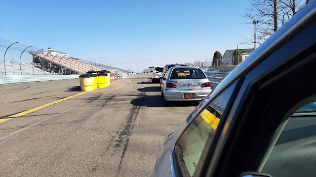
This sloped extension was built to test for attached flow and pressure recovery. However, it is only an initial approximation—a model—of a full tail on this car.

And how do we know if the model is good enough to predict the real thing? How close is “good enough”? Well, determination of the fidelity of models, gauging the impact of our assumptions, deciding to throw out some parameters as negligible—all these fall under the purview of “engineering judgment.” That only comes with experience. Next time, we’ll look at an example of real world testing and compare it to a simple numerical model as a way to build that experience.

Previous: Why Your CFD Is Wrong – Part 1: What Is a Model?